Exploring the Data

In the last post, I introduced the goals of this project. In this post, I’ll start taking a closer look at the data. At this point, I have data from 55 flights at two hang gliding sites.

My vario produces kmz files, which contain XML that can be parsed for timestamp and positional data (latitude, longitude, altitude). Sample raw data is shown below.

...
<when>2018-10-14T18:26:03Z</when>
<gx:coord>-79.479725 44.142231 300</gx:coord>
<when>2018-10-14T18:26:04Z</when>
<gx:coord>-79.479849 44.142214 305</gx:coord>
<when>2018-10-14T18:26:05Z</when>
<gx:coord>-79.479969 44.142205 311</gx:coord>
...

Developing a thermal predictor will involve deriving an underlying model of the flight characteristics of the glider from this data, as well as other sources of information (such as third party APIs for weather conditions and topographical information). This understanding will then be required to develop a model for thermal behaviour based on the various in-flight interactions with thermals contained within the dataset.

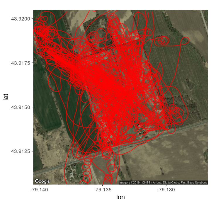
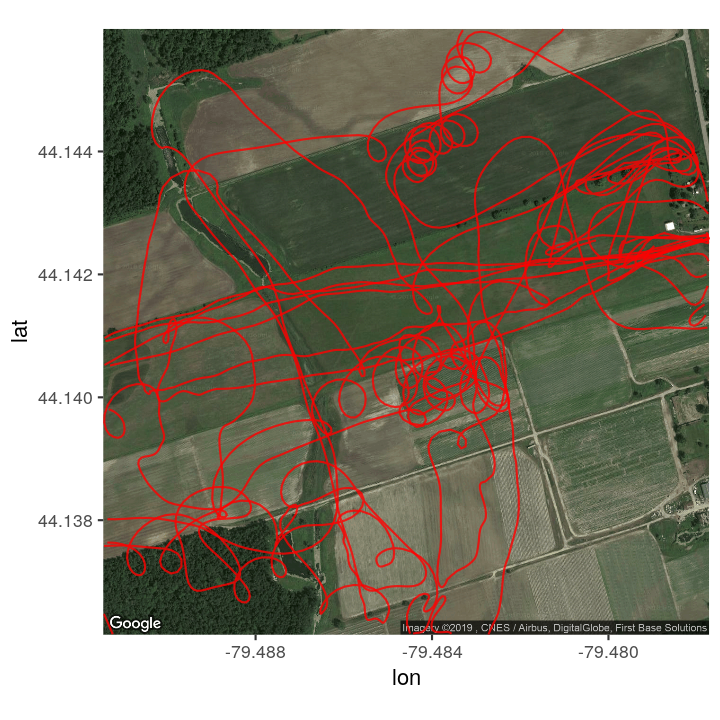
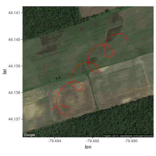
To begin to explore the data, I’ll start by looking at a specific flight to see what sort of information can be determined from the vario data. I chose the flight below, my first flight on Oct 14, 2018 (link). On this flight, there was a relatively strong wind from west-south-west, and I encountered a handful of thermals.

The long line from east to west indicates the tow, which involved a ground-based winch on the west end of the flight field.

Since the data contains both the altitude and a timestamp, it is straight-forward to plot altitude versus time to see the altitude profile of the flight.

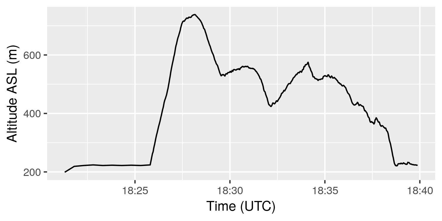
The plot shows the altitude as measured in meters above sea level. There is an initial period of inactivity, followed by a tow to altitude. After release, I encounter sink, but then find an area of lift, which I circle five times before losing it. I descend, then find stronger lift and climb again. The remainder of the flight, I encounter small pockets of lift, but am not able to successfully use any of them to gain altitude. The steep descent at the end of the flight is my landing approach.

There is no direct measure of speed or distance directly in the vario data. However these can be calculated. Using spherical trigonometry, we can get the distance between adjacent latitude-longitude pairs in the data, which can then be used to plot altitude as a function of cumulative flight distance. Technically this is assumes the travel occurs along a geodesic (or shortest path) between the adjacent points. When flying on curving path (such as circling in a thermal), the actual distance will be longer, however, this is a good enough approximation for now.

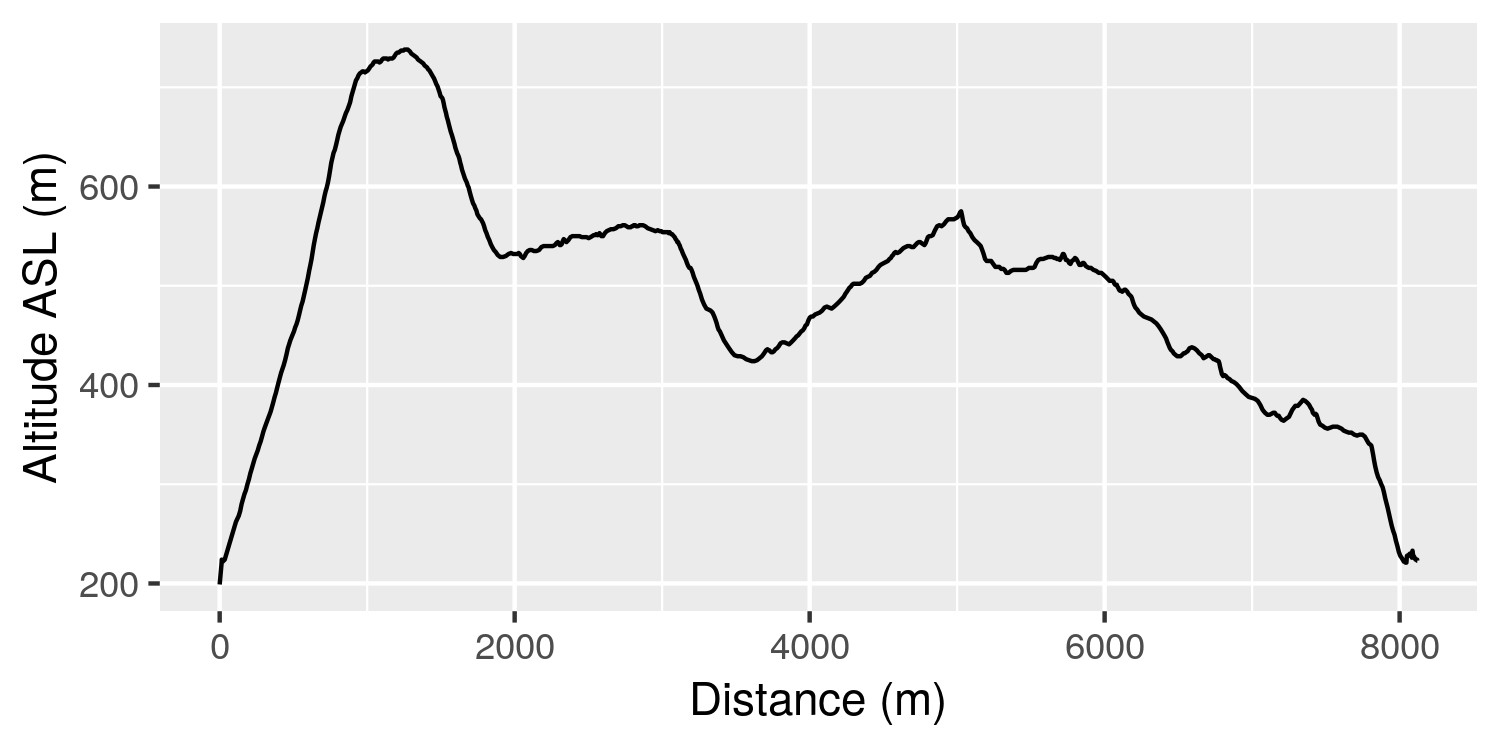
This plot is largely the same as the previous one, but is “stretched” or “squished” horizontally based on the speed of the glider. Since we now know distance, we can determine the ground speed between adjacent data points using,

\[ speed = distance / time \].

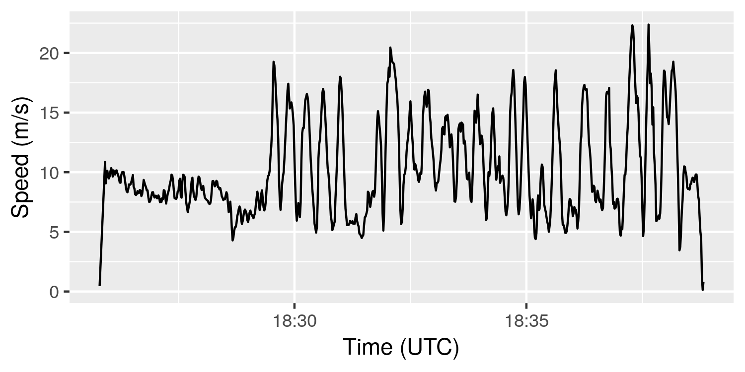
This plot shows an initial tow speed of approximately 8 m/s (29 kph). It then shows something interesting – a series of peaks and troughs, ranging between approximately 6 to 18 m/s (22 to 64 kph).

These patterns indicate that the glider is circling. Since the glider moves relative to the wind, the ground speed will increase when it is flying with the wind (tailwind), and decrease when flying into the wind (headwind). The plots below show two views of the same portion of the flight, with ground speed varying around an average speed of about 12 m/s (or 43 kph).

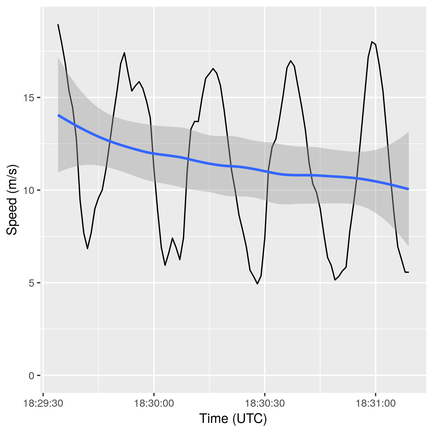
The vertical height between the peaks and troughs (i.e. the difference in speed) is related to the speed of the wind. The higher the wind speed, the more pronounced this effect will be. The wind speed will be (approximately) given by,

\[ (speed_{max}-speed_{min})/2 \]

Knowing the wind speed will be incredibly useful in understanding the glider flight characteristics. Based on the findings above, it seems likely that it will be possible to estimate the wind speed from the vario flight data. However, wind direction is also important.

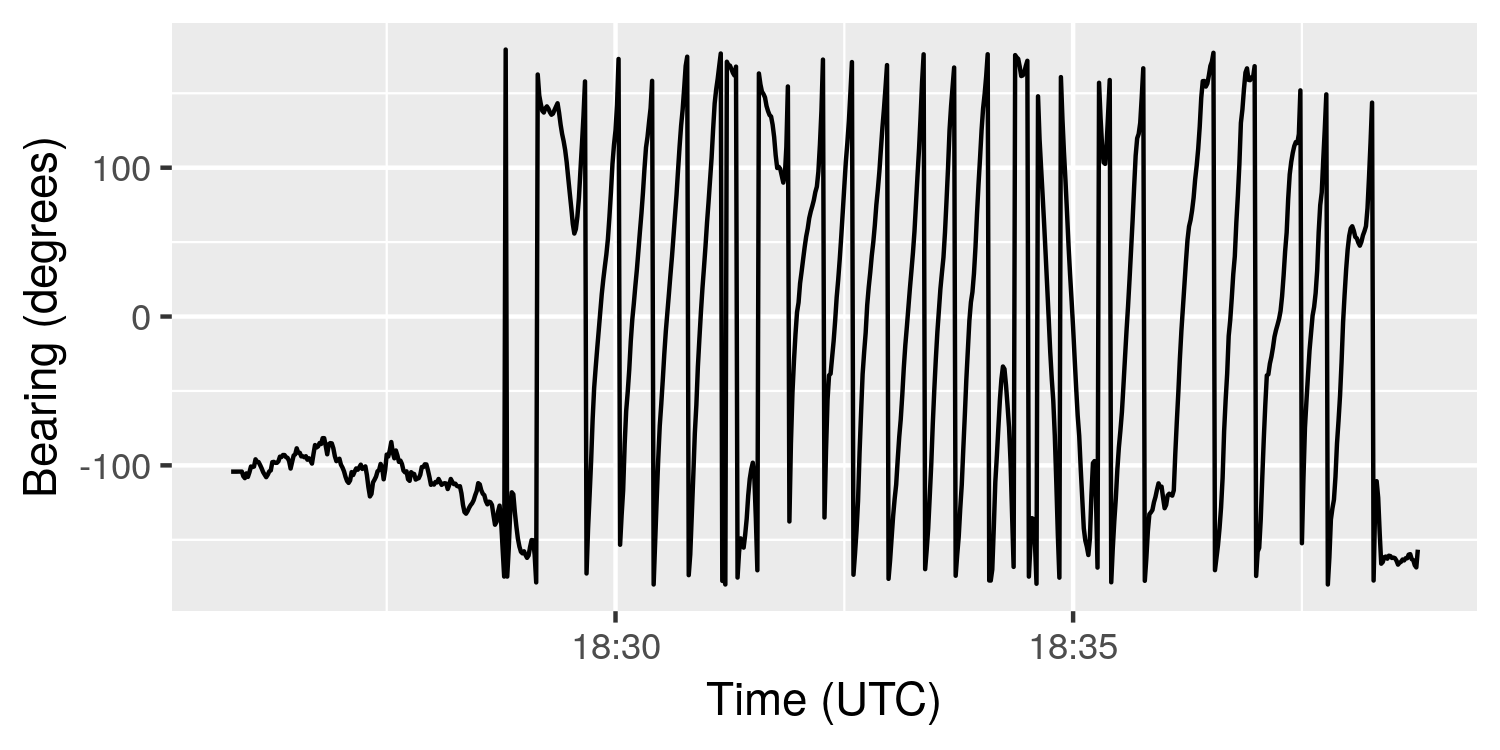
We can determine the direction of travel by resorting once again to math. Using the latitude and longitude data, we can calculate the bearing, or direction of travel between two points. Note that this is not necessarily the direction that the glider is pointing, but just the direction is is moving relative to the ground.

The plot below shows the bearing of the glider over the course of the flight (in degrees ranging from -180 to 180, with zero being North). There is a period of travel in one direction (during tow), and then most of the flight is spent circling. At the end of the flight, the glider turns to face into the wind, since landing in a headwind reduces ground speed. Assuming the pilot does this correctly (and most of the time they do), the direction at landing gives a very good after-the-fact indication of the wind direction at low altitude.

The plot below shows the speed of the glider vs the bearing using polar coordinates for a small portion of circling within a thermal (the same portion which was shown in the preceding side-by-side figures). The distance from the center of the plot indicates ground speed, and the angle from the center indicates the bearing.

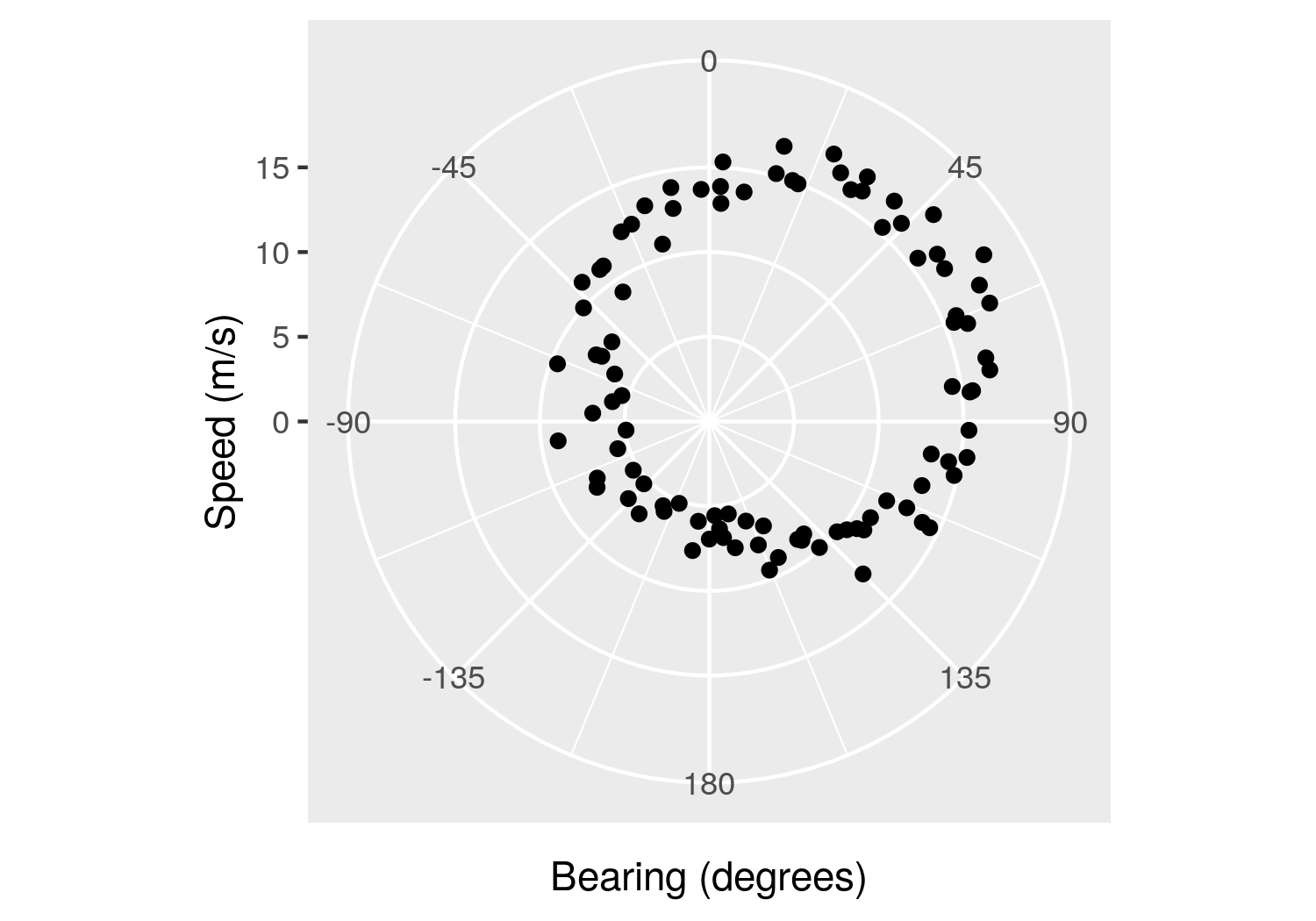
This is cool stuff! The plot shows a circle, which is offset from the center of the plot (up and to the right). This is because the glider is circling while being pushed along by the wind, resulting in the translation of all of the points. Assuming the glider’s circling is reasonably uniform, the center of this circle gives both the speed and direction of the wind. (The radius of the circle is related to the speed of the glider, and the “thickness” of the circular band is related to the range of airspeeds encountered during that portion of the glide.)

The plot above suggests that a few smooth circles should be sufficient to determine current wind speed and direction at a given altitude with reasonable accuracy. It is worth noting that hang-gliding is a sport that involves lots of flying in circles. Additionally, using assumptions about characteristic glider airspeeds, it may be possible to use a similar process to estimate the wind speed and direction using straight-line travel in a handful of directions and “extrapolating” the circle.

Variometers are typically equipped to provide audible feedback to indicate whether a glider is in a thermal. A method that many varios use when determining whether to provide the audible “you’re-going-up” tone, is total energy compensation. The purpose of this is to avoid confusing real thermals with “stick thermals”, which is when a glider pilot trades speed for altitude by pushing out on the control bar. The idea is that the total energy (kinetic and potential) of the glider is considered, so that trading altitude for speed or speed for altitude is accounted for.

\[ E_{total} = E_{potential} + E_{kinetic} = mgh + \frac{1}{2}mV^2 \]

Since gliders are not powered, they trade altitude (\(E_{potential}\)) for speed (\(E_{kinetic}\)), some of which is continually lost to drag. So in the absence of any external forces, \(E_{total}\) will gradually decrease despite any trade-offs between \(E_{potential}\) and \(E_{kinetic}\). Any increase in \(E_{total}\), then, must be from an external force (e.g., an increase in \(E_{potential}\) from a rising thermal, or an increase in \(E_{kinetic}\) from getting hit by an airplane). Using total energy is a more accurate way to determine the presence of thermals than the change in altitude alone.

The \(V\) in the equation above is for airspeed. However, we haven’t solved for that yet, so I’ll cheat a little and use ground speed. Further, to avoid the need to calculate mass term \(m\), I’ll divide it out of the equation to use the specific energy (energy per unit mass). Doing this gives the plot below.

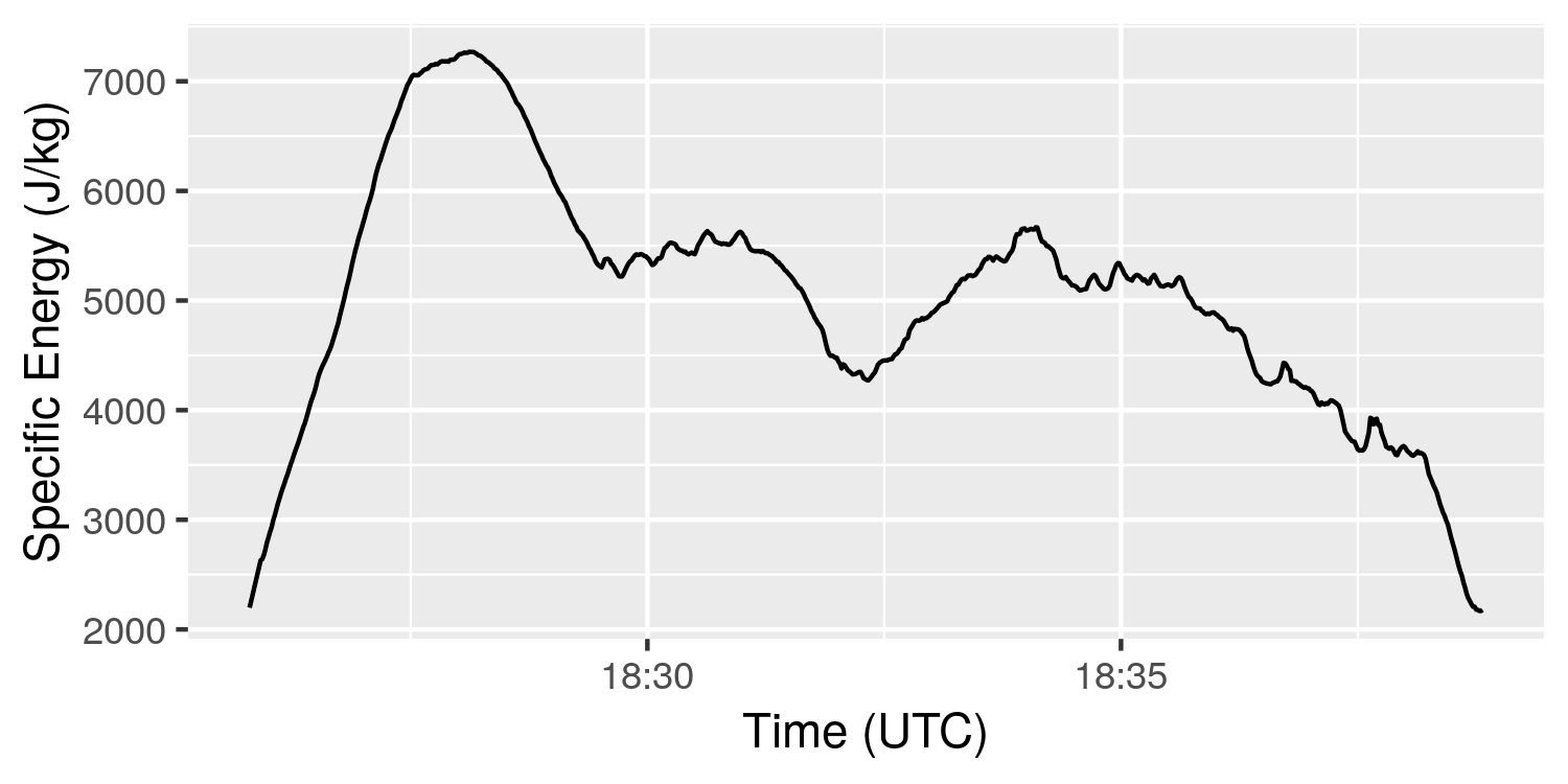
Clearly, the specific energy is dominated by the potential energy component (i.e. the altitude). Looking at only the rate of change of the specific energy gives the plot below.

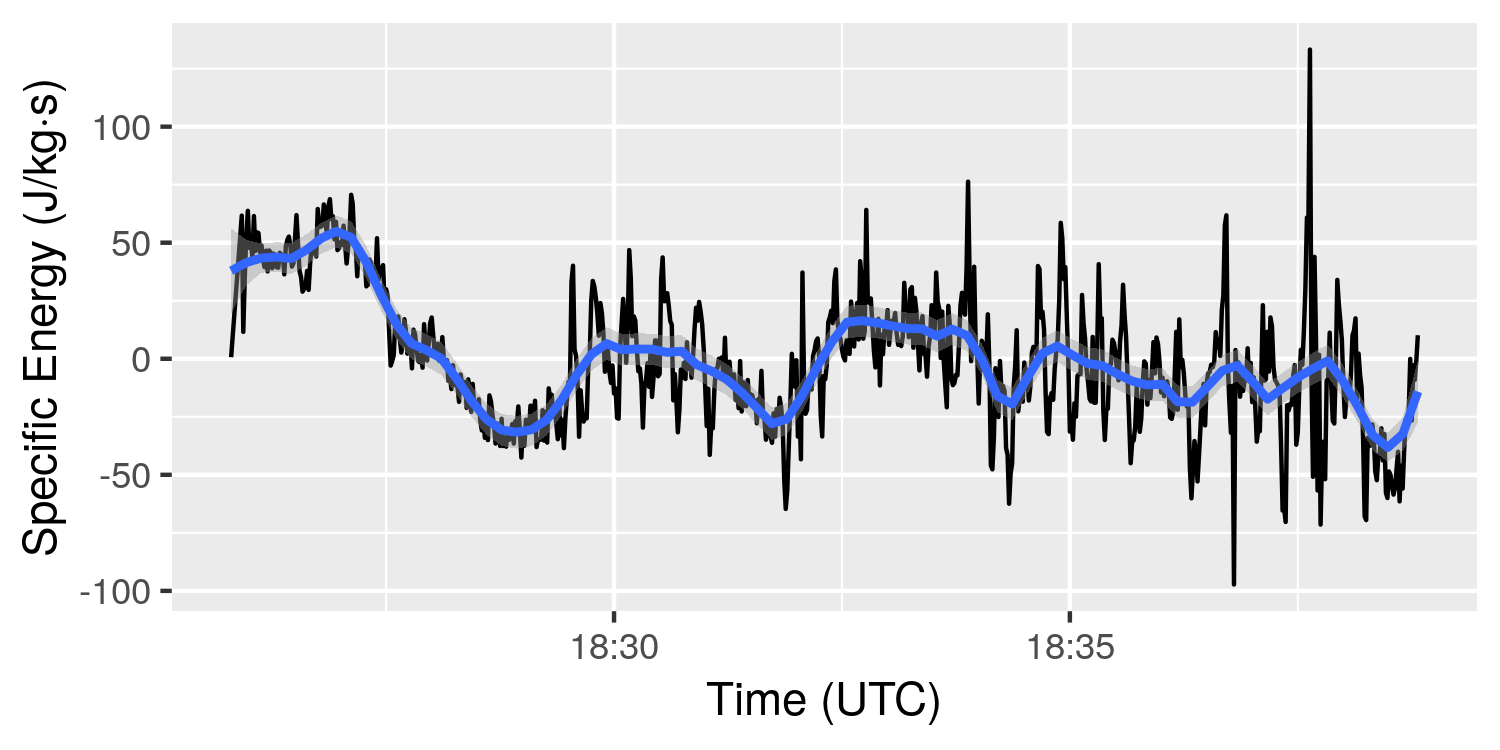
The plot shows a positive value of about 50 J/kg under tow, with the remainder of the flight generally being slightly negative, as expected. The “wobbles” visible in both plots (the vertical noise when circling is occurring), are a result of the decision to use ground speed instead of airspeed in the calculation. These should not be there, since the glider is not actually speeding up and slowing down with each circle. In reality, the plotted data should be closer to the smoothed blue curve, which generally is above zero if the glider is in lift, and below zero if not.

A good estimate of the wind speed and direction could be used to approximate airspeed. When this is done, the vertical “wobbles” in the plots above would be expected to essentially disappear. In fact, it might be possible to approximate wind speed and direction simply by finding the solution that minimizes the “wobbles” on the plot above.

In any case, obtaining a reasonable approximation of wind speed and direction is going to be very important, as the behaviour of both the glider and thermals depend on it. Further, it will be important that the wind speed and direction are updated throughout the flight, since they vary with location, altitude, and time. Having a reasonable approximation of the wind profile all the way to the ground may help to identify surface features which are correlated with thermals under particular conditions. It may then be possible to use this learned information to predict where thermals may occur based on current flight conditions.

Next steps will include:

• Continue to develop an understanding of the glider flight characteristics.
• Develop ways to characterize different flight modes, for instance, under-tow or gliding. When using the data to develop a model of flight behaviour, it will be important to extract only the portions where the glider is in free flight (i.e. not under tow). Extracting the relevant flight data will need to be done programmatically so that it can scale for any number of flight data logs.
• Build parsers for additional data formats, as not all varios output the same file format. Further, there are many additional flights were I have cellphone sensor dump data. This includes time, GPS location, and barometric pressure (which can be used to approximate altitude). Knowing the quality of this data will be useful since a cellphone app would be a good method for deploying an in-flight recommendation system for finding thermals.